Hello, this is about the complete flow for a regression machine learning solution. EDA — Exploratory Data Analysis is the first step towards any machine learning problem. It is about understanding the data before moving further. It goes like understand the problem first and then solve it. I feel more time spent on data more comfortable you become towards solving ML problems. Dataset used in this can be found here[0]. All are floating-point values. I have covered almost all the regression models in Sklearn and using GrdidsearchCV. GridsearchCV finds the best possible model parameters and it implements score on the cross-validation which is a measure of the model. Also to make it a little interesting, have covered almost all preprocessing techniques for scaling.
The idea behind this experiment is, it is not possible to master all the techniques in a short amount of time. To bypass this time of not understanding all the techniques in-depth, run this method to give an insight into which method to look into and pick like best three or five combinations and analyze more on the same if needed. Also to avoid all the doubts in mind why not try other combinations. This will give an idea as to what is the thing that you have got in front of you to solve a given problem.
Code for this is divided into three-part:
EDA — Exploratory Data Analytics
As I have said in the intro it is very vital dealing with ML. By doing this you almost end up yourself thinking about which ML model that you want to use for this. More time you spend more insights and problems you will see and start finding solutions to tackle it. This mainly involves below points:
- Data Distribution
- Outliers Involved
- Analyzing Categorical / Numerical features(Some numerical features are also categorical)
- Data Imputation
- Dimensionality Reduction — PCA (Feature selection if not deep learning)
Data distribution is understanding how each feature is varied, is it too random? is it uniform? is it uniform with outliers? how many missing values for each feature? This is understood with pandas describe. This gives mean, median, std, and percentiles 25, 50 and 75. Standard deviation is a measure of spread. How the numeric feature is spread out? If the value is high it is a clear indication that data is spread out on a wider range. A very good video on youtube to understand all these parameters.

Doing analysis for a few features:
age: total count is clear(i.e there is 2100 entry in the table and of course it should be the same for all features). mean is 64.4 this says that the average age of consideration is 64.4, from that you can get an idea like if there is an entry with age below 10 you might get some doubt if the data is correct or wrong. This is the measure of correctness in my terms with the help of standard deviation. std is 9.1 so this looks fine, it is not a very big number. It should be less for ideal datasets. This says that from mean that is 64.4 a regular data can vary in the range of 9.1. So if you see any data varying badly from mean with respect to std then it can be considered as an outlier and has to be understood properly before taking any action on such data.
test_time: source says(test_time — Time since recruitment into the trial. The integer part is the number of days since recruitment[0]) from this we can say, either it should be zero or a positive integer. But there are few negative values. This can be tackled in many ways, I have done one of the experiments in this Colab by replacing it with mean value, but didn't make much of a difference, as there are only 3 negative values. Here again, std is around 53 which is a little more, so it can be assumed distribution will be wider, and max value and .75 percentile value has a big difference as well, leading us to assume to have more outliers.
For Outliers and Imputation please follow this article. And categorical should be converted to numerical representation by methods like one-hot encoding. It is always better to use one-hot encode rather than replacing it with a sequence of numbers(1, 2, 3, etc) which may introduce bias.
By the above steps, like one hot encoding along with numerical values, might increase features by many. So in order to keep features that really matter for the prediction, features with low relevance for prediction should be filtered out. If not training will takes ages to complete unless the infrastructure is very good. PCA is one of the well-known dimensionality reduction techniques. There are many videos on youtube. My suggestion would be this.
GridSearchCV:
This is another good friend from sklearn community, it does all the hard work of trying it out many different combinations that we specify. GridSearchCV is like a developer and hyperparameters are the commands of his manager. Developers do all the work based on the hyperparameters. Like how different developer s need to be tackled differently with different motivation factors, even for GridSearchCV needs this different motivation on different MachineLearning models. All this hyperparameter that I feel is enough or known in the model_list.py file. It is like a configuration file that can be changed anytime for any purpose. More details from Skelarn.
Preprocessing
Preprocessing as said above done to give equal importance for each feature. Sklearn has defined many preprocessing techniques, in this exercise I have tried 8 different scaling method. Once this preprocessing is done new CSV is created out of it. All this is done after data analysis done on the original data. And each dataset is run against 15 machine learning models. Each result is then stored and further analysis is done on this result. This is available in the final Colab.
So this is how the code is to be used: Final part →framework →Analysis.
Once the Analysis is done for a given problem replace the model in the final part. In the Framework, there is a very good way of understanding each feature. The framework mainly has three functions:
- generate_csv_with_different_scaling_method: generate CSV for each scaling method
- analyse_distribution: This generates an image in the image path
- cluster_analysis: This gives cluster analysis image in cluster path
- train: This run iterations over CSV’s and models.
This concludes my experiment. From the Analysis, I found out for the regression dataset mentioned above RandomForestRegressor is the best and has performed across the scaling method. This is not generic enough to handle all type of datasets, going further will update. I would like to hear if any thoughts on this and I hope it helps others as this involves the complete process of machine learning. Enjoy sharing!!! Enjoy Coding!!!
References:
[0] Athanasios Tsanas, Max A. Little, Patrick E. McSharry, Lorraine O. Ramig (2009),’Accurate telemonitoring of Parkinson’s disease progression by non-invasive speech tests’, IEEE Transactions on Biomedical Engineering (to appear).